Numpy Overview
Please Log In for full access to the web site.
Note that this link will take you to an external site (https://shimmer.mit.edu) to authenticate, and then you will be redirected back to this page.
Most of this numpy overview reference material was taken from here. Here are some more handy reference sheets:
numpy is a package for doing a variety of numerical computations in Python. We will use it extensively. It supports writing very compact and efficient code for handling arrays of data. We will start every code file that uses numpy with import numpy as np, so that we can reference numpy functions with the 'np.' precedent.
IMPORTANT NOTE about INDEXING FAILURES. In 6.390, we always work with 2D arrays. Numpy indexing can sometimes collapse a dimension. To avoid this, make sure that you always provide a range of indices, even if you want to extract just one. This might look something like A[i:i+1, j:j+1] to extract the value at indices (i, j) in matrix A in the form of a 2D array. Failure to do so may make numpy crash - or worse, fail in silent ways.
Creating Arrays
Numpy arrays are homogeneous in nature, i.e., they comprise one data type (integer, float, double, etc.) unlike lists.
# There are many ways to create arrays, here are a few:
# creating a length 10 1D array of all zeros
>>> np.zeros(10, dtype='int')
np.array([0, 0, 0, 0, 0, 0, 0, 0, 0, 0])

# creating a 3 row x 5 column matrix
>>> np.ones((3,5), dtype=float)
np.array([[ 1.,  1.,  1.,  1.,  1.],
      [ 1.,  1.,  1.,  1.,  1.],
      [ 1.,  1.,  1.,  1.,  1.]])


# creating a matrix with a predefined value
>>> np.full((3,5),1.23)
np.array([[ 1.23,  1.23,  1.23,  1.23,  1.23],
      [ 1.23,  1.23,  1.23,  1.23,  1.23],
      [ 1.23,  1.23,  1.23,  1.23,  1.23]])

# create an array with a set sequence
>>> np.arange(0, 20, 2)
np.array([0, 2, 4, 6, 8,10,12,14,16,18])

# create an array of even space between the given range of values
>>> np.linspace(0, 1, 5)
np.array([ 0., 0.25, 0.5 , 0.75, 1.])

# create a 3x3 array with mean 0 and standard deviation 1 in a given dimension
>>> np.random.normal(0, 1, (3,3))
np.array([[ 0.72432142, -0.90024075,  0.27363808],
      [ 0.88426129,  1.45096856, -1.03547109],
      [-0.42930994, -1.02284441, -1.59753603]])

# create an identity matrix
>>> np.eye(3)
np.array([[ 1.,  0.,  0.],
      [ 0.,  1.,  0.],
      [ 0.,  0.,  1.]])

# set a random seed
>>> np.random.seed(0)

>>> x1 = np.random.randint(10, size=6) #one dimension
>>> x2 = np.random.randint(10, size=(3,4)) #two dimension
>>> x3 = np.random.randint(10, size=(3,4,5)) #three dimension

>>> print("x3 ndim:", x3.ndim)
('x3 ndim:', 3)
>>> print("x3 shape:", x3.shape)
('x3 shape:', (3, 4, 5))
>>> print("x3 size: ", x3.size)
('x3 size: ', 60)
Array Indexing
Remember: python indexing starts at zero.
# Creating an np.array with a python list
>>> x1 = np.array([4, 3, 4, 4, 8, 4])
>>> x1
np.array([4, 3, 4, 4, 8, 4])

# assess value at index zero
>>> x1[0]
4

# assess fifth value
>>> x1[4]
8

# get the last value
>>> x1[-1]
4

# get the second last value
>>> x1[-2]
8

# in a multidimensional array, we need to specify row and column index
>>> x2 = np.array([[3, 7, 5, 5],
                    [0, 1, 5, 9],
                    [3, 0, 5, 0]])

# 3rd row and 4th column value
>>> x2[2,3]
0

# Last value of the values within the 3rd row
>>> x2[2,-1]
0

# replace value at 0,0 index
>>> x2[0,0] = 12
>>> x2
np.array([[12,  7,  5,  5],
      [ 0,  1,  5,  9],
      [ 3,  0,  5,  0]])
Array Slicing - 1D
Now, we'll learn to access multiple or a range of elements from an array.
>>> x = np.arange(10)
>>> x
np.array([0, 1, 2, 3, 4, 5, 6, 7, 8, 9])

# from start to the 5th value, inclusive
>>> x[:5]
np.array([0, 1, 2, 3, 4])

# from the 5th value to the end, inclusive
>>> x[4:]
np.array([4, 5, 6, 7, 8, 9])

# the 5th through the 7th value, inclusive
>>> x[4:7]
np.array([4, 5, 6])

# return elements at even places
>>> x[ : : 2]
np.array([0, 2, 4, 6, 8])

# return elements from first position step by two
>>> x[1::2]
np.array([1, 3, 5, 7, 9])

# reverse the array
>>> x[::-1]
np.array([9, 8, 7, 6, 5, 4, 3, 2, 1, 0])
Array Slicing - MULTI-DIMENSIONAL
Now, let’s access multiple or a range of elements from a numpy (multidimensional) ndarray.
>>> x = np.arange(10).reshape(2,5)
>>> x
np.array([[0, 1, 2, 3, 4],
          [5, 6, 7, 8, 9]])

#  Grab all rows, column 2, return a 1D array (LOSE A DIMENSION!)
#  np.array([[0, 1, 2, 3, 4],
#           [5, 6, 7, 8, 9]])
>>> x[:,2]
np.array([2,7])

#  Grab all rows, column 2, return a 2D array (preserve dimension)
#  np.array([[0, 1, 2, 3, 4],
#           [5, 6, 7, 8, 9]])
>>> x[:,2:3]
array([[2],
       [7]])
#  OR
>>> x[:,[2]]
array([[2],
       [7]])

#  Grab all rows, columns 2 through 4 (not including column 4), return a 2D array (preserve dimension)
#  np.array([[0, 1, 2, 3, 4],
#           [5, 6, 7, 8, 9]])
>>> x[:,2:4]
np.array([[2, 3],
          [7, 8]])
#  OR
>>> x[:,[2,3]]
np.array([[2, 3],
          [7, 8]])

#  Grab all rows, columns 0 and 3, return a 2D array (preserve dimension)
#  np.array([[0, 1, 2, 3, 4],
#           [5, 6, 7, 8, 9]])
>>> x[:,[0,3]]
np.array([[0, 3],
          [5, 8]])
Everything above can work for rows just as easily as columns.
Array Concatenation
Many a time, we are required to combine different arrays. So, instead of typing each of their elements manually, you can use array concatenation to handle such tasks easily.
# You can concatenate two or more arrays at once.
>>> x = np.array([1, 2, 3])
>>> y = np.array([3, 2, 1])
>>> z = [21,21,21]
>>> np.concatenate([x, y, z])
np.array([ 1,  2,  3,  3,  2,  1, 21, 21, 21])

# You can also use this function to create 2-dimensional arrays.
>>> grid = np.array([[1,2,3],[4,5,6]])
>>> np.concatenate([grid, grid])
np.array([[1, 2, 3],
      [4, 5, 6],
      [1, 2, 3],
      [4, 5, 6]])

# Using its axis parameter, you can define row-wise or column-wise matrix
>>> np.concatenate([grid, grid], axis=1)
np.array([[1, 2, 3, 1, 2, 3],
      [4, 5, 6, 4, 5, 6]])
Until now, we used the concatenation function of arrays of equal dimension. But, what if you are required to combine a 2D array with 1D array? In such situations, np.concatenate might not be the best option to use. Instead, you can use np.vstack or np.hstack to do the task. Let's see how!
>>> x = np.array([3,4,5])
>>> grid = np.array([[1,2,3],[17,18,19]])
>>> np.vstack([x, grid])
np.array([[ 3,  4,  5],
      [ 1,  2,  3],
      [17, 18, 19]])

# Similarly, you can add an array using np.hstack
>>> z = np.array([[9],[9]])
>>> np.hstack([grid, z])
np.array([[ 1,  2,  3,  9],
      [17, 18, 19,  9]])
Also, we can split the arrays based on pre-defined positions. Let's see how!
>>> x = np.arange(10)
>>> x
np.array([0, 1, 2, 3, 4, 5, 6, 7, 8, 9])

>>> x1,x2,x3 = np.split(x,[3,6])
>>> print(x1,x2,x3)
[0 1 2] [3 4 5] [6 7 8 9]

>>> grid = np.arange(16).reshape((4,4))
>>> grid
>>> upper, lower = np.vsplit(grid,[2])
>>> print (upper, lower)
(np.array([[0, 1, 2, 3],
       [4, 5, 6, 7]]), np.array([[ 8,  9, 10, 11],
       [12, 13, 14, 15]]))
Broadcasting
What is Broadcasting?
Broadcasting is a numpy feature that repeats arithmetic operations like +, -, x, and ÷ between smaller and a larger numpy arrays. Examples:
- Add/Sub/Mul/Div a scalar with every element of an entire vector or matrix.
>>> scalar = 10
>>> vector = np.array([0, 1, 2, 3])
>>> scalar + vector
np.array([10, 11, 12, 13])
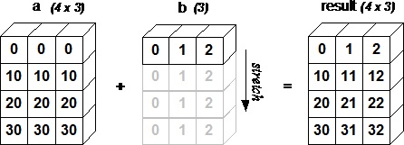
- Add/Sub/Mul/Div a vector with every row of a matrix.
>>> matrix = np.array([[0, 1, 2, 3],
                       [4, 5, 6, 7]])
>>> vector + matrix
np.array([[0, 2, 4, 6],
          [4, 6, 8, 10]])
- Add/Sub/Mul/Div a vector with every column of a matrix.
>>> column = np.array([-10,10]).reshape((2,1))
>>> column + matrix
np.array([[-10, -9, -8, -7],
          [14, 15, 16, 17]])
Syntax is identical to arithmetic with two scalars: operand_1 <operation> operand_2 ... if your operands have proper shapes!
Proper Broadcasting shapes
When operating on two arrays, NumPy compares their shapes element-wise. It starts with the trailing dimensions, and works its way forward. Two dimensions are compatible when:
- they are equal, or
- one of them is 1
Visual Example:
Examples of Shapes That Broadcast
A      (2d array):  5 x 4
B      (1d array):      1
Result (2d array):  5 x 4

A      (2d array):  5 x 4
B      (1d array):      4
Result (2d array):  5 x 4

A      (3d array):  15 x 3 x 5
B      (3d array):  15 x 1 x 5
Result (3d array):  15 x 3 x 5

A      (3d array):  15 x 3 x 5
B      (2d array):       3 x 5
Result (3d array):  15 x 3 x 5

A      (3d array):  15 x 3 x 5
B      (2d array):       3 x 1
Result (3d array):  15 x 3 x 5
Examples of Shapes That Don't Broadcast
A      (1d array):  3
B      (1d array):  4 # trailing dimensions do not match

A      (2d array):      2 x 1
B      (3d array):  8 x 4 x 3 # second from last dimensions mismatched