7 Convolutional Neural Networks
So far, we have studied what are called fully connected neural networks, in which all of the units in one layer are connected to all of the units in the next layer. This is a good arrangement when we don’t know anything about the kind of mapping from inputs to outputs that we will be asking the network to approximate. However, if we do know something about our problem, it is better to build that knowledge into the structure of the neural network. Doing so can save computation time and significantly reduce the amount of training data required to arrive at a solution that generalizes robustly.
One very important application domain of neural networks, where these methods have achieved an enormous amount of success in recent years, is signal processing. Signals may be spatial (as in two-dimensional camera images or three-dimensional depth or CAT scans) or temporal (such as speech or music). If we know that we are addressing a signal-processing problem, we can take advantage of its invariant properties. In this chapter, we will focus on two-dimensional spatial problems (images), using one-dimensional examples for simplicity. In a later chapter, we will address temporal problems.
Imagine that you are given the task of designing and training a neural network that takes an image as input and outputs a classification that is positive if the image contains a cat and negative if it does not. An image can be described as a two-dimensional array of pixels, each of which may be represented by three integer values, encoding intensity levels in the red, green, and blue color channels.
A pixel is a “picture element.”
There are two important pieces of prior structural knowledge we can bring to bear on this problem:
- Spatial locality: The set of pixels we will have to take into consideration to find a cat will be near one another in the image.
So, for example, we won’t have to consider some combination of pixels in the four corners of the image, in order to see if they encode cat-ness.
- Translation invariance: The pattern of pixels that characterizes a cat is the same no matter where in the image the cat occurs.
Cats don’t look different if they’re on the left or the right side of the image.
We will design neural network structures that take advantage of these properties.
7.1 Filters
We begin by discussing image filters.
Unfortunately in AI/ML/CS/Math, the word ``filter’’ gets used in many ways: in addition to the one we describe here, it can describe a temporal process (in fact, our moving averages are a kind of filter) and even a somewhat esoteric algebraic structure.
An image filter is a function that takes in a local spatial neighborhood of pixel values and detects the presence of some pattern in that data.
Let’s consider a very simple case to start, in which we have a 1-dimensional binary “image” and a filter \(F\) of size two. The filter is a vector of two numbers, which we will move along the image, taking the dot product between the filter values and the image values at each step, and aggregating the outputs to produce a new image.
Let \(X\) be the original image, of size \(d\); then pixel \(i\) of the output image is specified by \[Y_i = F \cdot (X_{i-1}, X_i)\;\;.\] To ensure that the output image is also of dimension \(d\), we will generally “pad” the input image with 0 values if we need to access pixels that are beyond the bounds of the input image. This process of applying the filter to the image to create a new image is called “convolution.”
And filters are also sometimes called convolutional kernels.
If you are already familiar with what a convolution is, you might notice that this definition corresponds to what is often called a correlation and not to a convolution. Indeed, correlation and convolution refer to different operations in signal processing. However, in the neural networks literature, most libraries implement the correlation (as described in this chapter) but call it convolution. The distinction is not significant; in principle, if convolution is required to solve the problem, the network could learn the necessary weights. For a discussion of the difference between convolution and correlation and the conventions used in the literature you can read Section 9.1 in this excellent book: Deep Learning.
Here is a concrete example. Let the filter \(F_1 = (-1, +1)\). Then given the image in the first line below, we can convolve it with filter \(F_1\) to obtain the second image. You can think of this filter as a detector for “left edges” in the original image—to see this, look at the places where there is a \(1\) in the output image, and see what pattern exists at that position in the input image. Another interesting filter is \(F_2 = (-1, +1, -1)\). The third image (the last line below) shows the result of convolving the first image with \(F_2\), where we see that the output pixel \(i\) corresponds to when the center of \(F_2\) is aligned at input pixel \(i\).
Convince yourself that filter \(F_2\) can be understood as a detector for isolated positive pixels in the binary image.
 grid (10, 1);
\setcounter{col}{1}
\foreach \p in {0,0,1,1,1,0,1,0,0,0} {
\edef\x{\value{col} - 0.5}
\node[anchor=center] at (\x, 0.5) {\p};
\stepcounter{col}
}
\node[left] at (0,0.5) {Image:};
\draw (0, -2) grid (2, -1);
\node[left] at (0, -1.5) {$F_1$:};
\node[anchor=center] (f11) at (0.5, -1.5) {-1};
\node[anchor=center] (f12) at (1.5, -1.5) {+1};
\coordinate (x1) at (0.5, 0);
\coordinate (x2) at (1.5, 0);
\draw[->] (x1) -- ++(0,-1);
\draw[->] (x2) -- ++(0,-1);
\draw[->] (x1)++(0,-2) -- ++(1,-1);
\draw[->] (x2)++(0,-2) -- ++(0,-1);
\end{scope}
\begin{scope}[yshift=-2.8cm]
\draw (0, 0) grid (10, 1);
\setcounter{col}{1}
\foreach \p in {0,0,1,0,0,-1,1,-1,0,0} {
\edef\x{\value{col} - 0.5}
\node[anchor=center] at (\x, 0.5) {\p};
\stepcounter{col}
}
\node[left] at (0,0.5) {After convolution (with $F_1$):};
\draw[very thick] (2, 0) grid (3, 1);
\draw[very thick] (6, 0) grid (7, 1);
\end{scope}
\begin{scope}[yshift=-6.5cm]
\draw (0, 0) grid (10, 1);
\setcounter{col}{1}
\foreach \p in {0,-1,0,-1,0,-2,1,-1,0,0} {
\edef\x{\value{col} - 0.5}
\node[anchor=center] at (\x, 0.5) {\p};
\stepcounter{col}
}
\node[left] at (0,0.5) {After convolution (with $F_2$):};
\draw (0, 2) grid (3, 3);
\node[left] at (0, 2.5) {$F_2$};
\draw[very thick] (6, 0) grid (7, 1);
\node[anchor=center] at (0.5, 2.5) {-1};
\node[anchor=center] at (1.5, 2.5) {+1};
\node[anchor=center] at (2.5, 2.5) {-1};
\coordinate (x1) at (0.5, 4);
\coordinate (x2) at (1.5, 4);
\coordinate (x3) at (2.5, 4);
\draw[->] (x1)++(0,-0.5) -- ++(0,-0.5);
\draw[->] (x2)++(0,-0.5) -- ++(0,-0.5);
\draw[->] (x3)++(0,-0.5) -- ++(0,-0.5);
\draw[->] (x1)++(0,-2) -- ++(1,-1);
\draw[->] (x2)++(0,-2) -- ++(0,-1);
\draw[->] (x3)++(0,-2) -- ++(-1,-1);
\end{scope}
\end{tikzpicture}")
Two-dimensional versions of filters like these are thought to be found in the visual cortex of all mammalian brains. Similar patterns arise from statistical analysis of natural images. Computer vision people used to spend a lot of time hand-designing filter banks. A filter bank is a set of sets of filters, arranged as shown in the diagram below.
 rectangle (4,4);
\node[anchor=center] at (2,2) {Image};
% Arrows from image to filter stack
\foreach \yoff in {-1.2,-0.4,0.4,1.2} {
\draw[->,thick] (4.2,2) -- ++(1.3,\yoff);
}
% Filter bank - 3D stacked look (draw back to front)
% Each filter offset by (0.4, 0.4) for depth effect
\begin{scope}[shift={(6,0)}]
% Filter 4 (purple, back)
\begin{scope}[shift={(1.2, 1.2)}]
\fill[white] (0,0) rectangle (2,2);
\draw[step=4mm, color=purple, thick] (0,0) grid (2,2);
\draw[black,very thick] (0,0) rectangle (2,2);
\end{scope}
% Filter 3 (green)
\begin{scope}[shift={(0.8, 0.8)}]
\fill[white] (0,0) rectangle (2,2);
\draw[step=4mm, color=green!70!black, thick] (0,0) grid (2,2);
\draw[black,very thick] (0,0) rectangle (2,2);
\end{scope}
% Filter 2 (red)
\begin{scope}[shift={(0.4, 0.4)}]
\fill[white] (0,0) rectangle (2,2);
\draw[step=4mm, color=red, thick] (0,0) grid (2,2);
\draw[black,very thick] (0,0) rectangle (2,2);
\end{scope}
% Filter 1 (blue, front)
\fill[white] (0,0) rectangle (2,2);
\draw[step=4mm, color=blue, thick] (0,0) grid (2,2);
\draw[black,very thick] (0,0) rectangle (2,2);
\end{scope}
% Arrows from filter stack to channel stack
\foreach \yoff in {-1.2,-0.4,0.4,1.2} {
\draw[->,thick] (9.8,2) -- ++(1.3,\yoff);
}
% Feature maps - 3D stacked look (draw back to front)
\begin{scope}[shift={(11.6,-0.5)}]
% Channel 4 (purple, back)
\begin{scope}[shift={(1.2, 1.2)}]
\fill[white] (0,0) rectangle (3,3);
\draw[step=3mm, color=purple, thin] (0,0) grid (3,3);
\draw[black,very thick] (0,0) rectangle (3,3);
\end{scope}
% Channel 3 (green)
\begin{scope}[shift={(0.8, 0.8)}]
\fill[white] (0,0) rectangle (3,3);
\draw[step=3mm, color=green!70!black, thin] (0,0) grid (3,3);
\draw[black,very thick] (0,0) rectangle (3,3);
\end{scope}
% Channel 2 (red)
\begin{scope}[shift={(0.4, 0.4)}]
\fill[white] (0,0) rectangle (3,3);
\draw[step=3mm, color=red, thin] (0,0) grid (3,3);
\draw[black,very thick] (0,0) rectangle (3,3);
\end{scope}
% Channel 1 (blue, front)
\fill[white] (0,0) rectangle (3,3);
\draw[step=3mm, color=blue, thin] (0,0) grid (3,3);
\draw[black,very thick] (0,0) rectangle (3,3);
\end{scope}
% Labels
\node[above] at (7.6,3.7) {Filter Bank};
\node[above] at (13.8,4.2) {Feature Maps};
\end{tikzpicture}")
All of the filters in the first group are applied to the original image; if there are \(k\) such filters, then the result is \(k\) new images, which are called channels. Now imagine stacking all these new images up so that we have a cube of data, indexed by the original row and column indices of the image, as well as by the channel. The next set of filters in the filter bank will generally be three-dimensional: each one will be applied to a sub-range of the row and column indices of the image and to all of the channels.
These 3D chunks of data are called tensors. The algebra of tensors is fun, and a lot like matrix algebra, but we won’t go into it in any detail.
There are now many useful neural-network software packages, such as TensorFlow and PyTorch that make operations on tensors easy.
Here is a more complex example of two-dimensional filtering. We have two \(3 \times 3\) filters in the first layer, \(f_1\) and \(f_2\). You can think of each one as “looking” for three pixels in a row, \(f_1\) vertically and \(f_2\) horizontally. Assuming our input image is \(n \times n\), then the result of filtering with these two filters is an \(n \times n \times 2\) tensor. Now we apply a tensor filter (hard to draw!) that “looks for” a combination of two horizontal and two vertical bars (now represented by individual pixels in the two channels), resulting in a single final \(n \times n\) image.
When we have a color image as input, we treat it as having three channels, and hence as an \(n \times n \times 3\) tensor.
Both slices of the tensor filter are identical here, so the output is simply the sum of the two channel values at each position.
 — cross pattern ===
\begin{scope}
\draw[black,thick] (0,0) grid (6,6);
\draw[black,very thick] (0,0) rectangle (6,6);
% Cross: vertical bar at x=3 (y=1..5), horizontal bar at y=3 (x=0..5)
\foreach \x/\y in {0/3,1/3,2/3,3/1,3/2,3/3,3/4,3/5,4/3,5/3} {
\fill[black] ($(\x,\y)$) rectangle ($(\x,\y)+(1,1)$);
\node[white] at ($(\x,\y)+(0.5,0.5)$) {1};
}
% 0 labels for non-black cells
\foreach \x in {0,1,2,4,5} {
\foreach \y in {0,1,2,4,5} {
\node at ($(\x,\y)+(0.5,0.5)$) {0};
}
}
\node at (3.5,0.5) {0};
\end{scope}
% === ARROWS FROM INPUT TO FILTERS ===
\draw[->,thick] (6.5,4.5) -- (8.5,8);
\draw[->,thick] (6.5,1.5) -- (8.5,-2);
% === f_2 (horizontal) FILTER at (9, 6.5) ===
\begin{scope}[shift={(9,6.5)}]
\draw[black,thick] (0,0) grid (3,3);
\draw[black,very thick] (0,0) rectangle (3,3);
\foreach \x/\y in {0/1,1/1,2/1} {
\fill[black] ($(\x,\y)$) rectangle ($(\x,\y)+(1,1)$);
\node[white] at ($(\x,\y)+(0.5,0.5)$) {1};
}
\foreach \x in {0,1,2} {
\foreach \y in {0,2} {
\node at ($(\x,\y)+(0.5,0.5)$) {0};
}
}
\node[above] at (1.5,3.3) {$f_2$ (horizontal)};
\end{scope}
% === f_1 (vertical) FILTER at (9, -4.5) ===
\begin{scope}[shift={(9,-4.5)}]
\draw[black,thick] (0,0) grid (3,3);
\draw[black,very thick] (0,0) rectangle (3,3);
\foreach \x/\y in {1/0,1/1,1/2} {
\fill[black] ($(\x,\y)$) rectangle ($(\x,\y)+(1,1)$);
\node[white] at ($(\x,\y)+(0.5,0.5)$) {1};
}
\foreach \x in {0,2} {
\foreach \y in {0,1,2} {
\node at ($(\x,\y)+(0.5,0.5)$) {0};
}
}
\node[below] at (1.5,-0.3) {$f_1$ (vertical)};
\end{scope}
% === ARROWS FROM FILTERS TO RESULTS ===
\draw[->,thick] (12.5,8) -- (14.5,8);
\draw[->,thick] (12.5,-3) -- (14.5,-3);
% === f_2 RESULT (horizontal detector) at (15, 5) ===
\begin{scope}[shift={(15,5)}]
\draw[black,thick] (0,0) grid (6,6);
\draw[black,very thick] (0,0) rectangle (6,6);
\node at (0.5,0.5) {0}; \node at (1.5,0.5) {0}; \node at (2.5,0.5) {0}; \node at (3.5,0.5) {0}; \node at (4.5,0.5) {0}; \node at (5.5,0.5) {0};
\node at (0.5,1.5) {0}; \node at (1.5,1.5) {0}; \node at (2.5,1.5) {1}; \node at (3.5,1.5) {1}; \node at (4.5,1.5) {1}; \node at (5.5,1.5) {0};
\node at (0.5,2.5) {0}; \node at (1.5,2.5) {0}; \node at (2.5,2.5) {1}; \node at (3.5,2.5) {1}; \node at (4.5,2.5) {1}; \node at (5.5,2.5) {0};
\node at (0.5,3.5) {2}; \node at (1.5,3.5) {3}; \node at (2.5,3.5) {3}; \node at (3.5,3.5) {3}; \node at (4.5,3.5) {3}; \node at (5.5,3.5) {2};
\node at (0.5,4.5) {0}; \node at (1.5,4.5) {0}; \node at (2.5,4.5) {1}; \node at (3.5,4.5) {1}; \node at (4.5,4.5) {1}; \node at (5.5,4.5) {0};
\node at (0.5,5.5) {0}; \node at (1.5,5.5) {0}; \node at (2.5,5.5) {1}; \node at (3.5,5.5) {1}; \node at (4.5,5.5) {1}; \node at (5.5,5.5) {0};
\end{scope}
% === f_1 RESULT (vertical detector) at (15, -6) ===
\begin{scope}[shift={(15,-6)}]
\draw[black,thick] (0,0) grid (6,6);
\draw[black,very thick] (0,0) rectangle (6,6);
\node at (0.5,0.5) {0}; \node at (1.5,0.5) {0}; \node at (2.5,0.5) {0}; \node at (3.5,0.5) {1}; \node at (4.5,0.5) {0}; \node at (5.5,0.5) {0};
\node at (0.5,1.5) {0}; \node at (1.5,1.5) {0}; \node at (2.5,1.5) {0}; \node at (3.5,1.5) {2}; \node at (4.5,1.5) {0}; \node at (5.5,1.5) {0};
\node at (0.5,2.5) {1}; \node at (1.5,2.5) {1}; \node at (2.5,2.5) {1}; \node at (3.5,2.5) {3}; \node at (4.5,2.5) {1}; \node at (5.5,2.5) {1};
\node at (0.5,3.5) {1}; \node at (1.5,3.5) {1}; \node at (2.5,3.5) {1}; \node at (3.5,3.5) {3}; \node at (4.5,3.5) {1}; \node at (5.5,3.5) {1};
\node at (0.5,4.5) {1}; \node at (1.5,4.5) {1}; \node at (2.5,4.5) {1}; \node at (3.5,4.5) {2}; \node at (4.5,4.5) {1}; \node at (5.5,4.5) {1};
\node at (0.5,5.5) {0}; \node at (1.5,5.5) {0}; \node at (2.5,5.5) {0}; \node at (3.5,5.5) {1}; \node at (4.5,5.5) {0}; \node at (5.5,5.5) {0};
\end{scope}
% === ARROWS FROM RESULTS TO TENSOR FILTER ===
\draw[->,thick] (21.5,8) -- (24.5,4);
\draw[->,thick] (21.5,-3) -- (24.5,2);
% === TENSOR FILTER at (25, 1.5) — two stacked 3x3 slices ===
\begin{scope}[shift={(25,1.5)}]
% Back slice (channel 2 / f_2)
\begin{scope}[shift={(0.5,0.5)}]
\fill[white] (0,0) rectangle (3,3);
\draw[black,thick] (0,0) grid (3,3);
\draw[black,very thick] (0,0) rectangle (3,3);
\node at (0.5,0.5) {0}; \node at (1.5,0.5) {0}; \node at (2.5,0.5) {0};
\node at (0.5,1.5) {0}; \node at (1.5,1.5) {1}; \node at (2.5,1.5) {0};
\node at (0.5,2.5) {0}; \node at (1.5,2.5) {0}; \node at (2.5,2.5) {0};
\end{scope}
% Front slice (channel 1 / f_1)
\fill[white] (0,0) rectangle (3,3);
\draw[black,thick] (0,0) grid (3,3);
\draw[black,very thick] (0,0) rectangle (3,3);
\node at (0.5,0.5) {0}; \node at (1.5,0.5) {0}; \node at (2.5,0.5) {0};
\node at (0.5,1.5) {0}; \node at (1.5,1.5) {1}; \node at (2.5,1.5) {0};
\node at (0.5,2.5) {0}; \node at (1.5,2.5) {0}; \node at (2.5,2.5) {0};
\node[above] at (1.75,3.8) {tensor filter};
\end{scope}
% === ARROW FROM TENSOR TO OUTPUT ===
\draw[->,thick] (29,3) -- (31,3);
% === FINAL OUTPUT at (31.5, 0) ===
\begin{scope}[shift={(31.5,0)}]
\draw[black,thick] (0,0) grid (6,6);
\draw[black,very thick] (0,0) rectangle (6,6);
\node at (0.5,0.5) {0}; \node at (1.5,0.5) {0}; \node at (2.5,0.5) {0}; \node at (3.5,0.5) {1}; \node at (4.5,0.5) {0}; \node at (5.5,0.5) {0};
\node at (0.5,1.5) {0}; \node at (1.5,1.5) {0}; \node at (2.5,1.5) {1}; \node at (3.5,1.5) {3}; \node at (4.5,1.5) {1}; \node at (5.5,1.5) {0};
\node at (0.5,2.5) {1}; \node at (1.5,2.5) {1}; \node at (2.5,2.5) {2}; \node at (3.5,2.5) {4}; \node at (4.5,2.5) {2}; \node at (5.5,2.5) {1};
\node at (0.5,3.5) {3}; \node at (1.5,3.5) {4}; \node at (2.5,3.5) {4}; \node at (3.5,3.5) {6}; \node at (4.5,3.5) {4}; \node at (5.5,3.5) {3};
\node at (0.5,4.5) {1}; \node at (1.5,4.5) {1}; \node at (2.5,4.5) {2}; \node at (3.5,4.5) {3}; \node at (4.5,4.5) {2}; \node at (5.5,4.5) {1};
\node at (0.5,5.5) {0}; \node at (1.5,5.5) {0}; \node at (2.5,5.5) {1}; \node at (3.5,5.5) {2}; \node at (4.5,5.5) {1}; \node at (5.5,5.5) {0};
\end{scope}
\end{tikzpicture}")
We are going to design neural networks that have this structure. Each “bank” of the filter bank will correspond to a neural-network layer. The numbers in the individual filters will be the “weights” (plus a single additive bias or offset value for each filter) of the network, that we will train using gradient descent. What makes this interesting and powerful (and somewhat confusing at first) is that the same weights are used many many times in the computation of each layer. This weight sharing means that we can express a transformation on a large image with relatively few parameters; it also means we’ll have to take care in figuring out exactly how to train it!
We will define a filter layer \(l\) formally with:
For simplicity, we are assuming that all images and filters are square (having the same number of rows and columns). That is in no way necessary, but is usually fine and definitely simplifies our notation.
number of filters \(m^l\);
size of one filter is \(k^l \times k^l \times m^{l-1}\) plus \(1\) bias value (for this one filter);
stride \(s^l\) is the spacing at which we apply the filter to the image; in all of our examples so far, we have used a stride of 1, but if we were to “skip” and apply the filter only at odd-numbered indices of the image, then it would have a stride of two (and produce a resulting image of half the size);
input tensor size \(n^{l-1} \times n^{l-1} \times m^{l-1}\)
padding: \(p^l\) is the addition of extra border values to an input before convolution to control output size and edge behavior. For an input of size \(n^{l-1} \times n^{l-1} \times m^{l-1}\), our new effective input size with padding becomes \((n^{l-1} + 2 \cdot p^l) \times (n^{l-1} + 2 \cdot p^l) \times m^{l-1}\).
This layer will produce an output tensor of size \(n^l \times n^l \times m^l\), where \(n^l = \lceil (n^{l-1} + 2 \cdot p^l - (k^l - 1)) / s^l \rceil\). The weights are the values defining the filter: there will be \(m^l\) different \(k^l \times k^l \times m^{l-1}\) tensors of weight values; plus each filter may have a bias term, which means there is one more weight value per filter. A filter with a bias operates just like the filter examples above, except we add the bias to the output. For instance, if we incorporated a bias term of 0.5 into the filter \(F_2\) above, the output would be \((-0.5,0.5,-0.5,0.5, -1.5, 1.5,-0.5,0.5)\) instead of \((-1,0,-1,0,-2,1,-1,0)\).
Recall that \(\lceil \cdot \rceil\) is the function; it returns the smallest integer greater than or equal to its input. E.g., \(\lceil 2.5 \rceil = 3\) and \(\lceil 3 \rceil = 3\).
This may seem complicated, but we get a rich class of mappings that exploit image structure and have many fewer weights than a fully connected layer would.
How many weights are in a convolutional layer specified as above?
If we used a fully-connected layer with the same size inputs and outputs, how many weights would it have?
7.2 Max pooling
It is typical (both in engineering and in nature) to structure filter banks into a pyramid, in which the image sizes get smaller in successive layers of processing. The idea is that we find local patterns, like bits of edges in the early layers, and then look for patterns in those patterns, etc. This means that, effectively, we are looking for patterns in larger pieces of the image as we apply successive filters. Having a stride greater than one makes the images smaller, but does not necessarily aggregate information over that spatial range.
Another common layer type, which accomplishes this aggregation, is max pooling. A max pooling layer operates like a filter, but has no weights. You can think of it as purely functional, like a ReLU in a fully connected network. It has a filter size, as in a filter layer, but simply returns the maximum value in its field.
We sometimes use the term receptive field or just field to mean the area of an input image that a filter is being applied to.
Usually, we apply max pooling with the following traits:
\(\text{stride} > 1\), so that the resulting image is smaller than the input image; and
\(k \geq \text{stride}\), so that the whole image is covered.
As a result of applying a max pooling layer, we don’t keep track of the precise location of a pattern. This helps our filters to learn to recognize patterns independent of their location.
Consider a max pooling layer where both the strides and \(k\) are set to be 2. This would map a \(64 \times 64 \times 3\) image to a \(32 \times 32 \times 3\) image. Note that max pooling layers do not have additional bias or offset values.
Maximilian Poole thinks it would be a good idea to add two max pooling layers of size \(k\), one right after the other, to their network. What single layer would be equivalent?
One potential concern about max-pooling layers is that they actually don’t completely preserve translation invariance. If you do max-pooling with a stride other than 1 (or just pool over the whole image size), then shifting the pattern you are hoping to detect within the image by a small amount can change the output of the max-pooling layer substantially, just because there are discontinuities induced by the way the max-pooling window matches up with its input image. Here is an interesting paper that illustrates this phenomenon clearly and suggests that one should first do max-pooling with a stride of 1, then do “downsampling” by averaging over a window of outputs.
7.3 Typical architecture
Here is the form of a typical convolutional network:
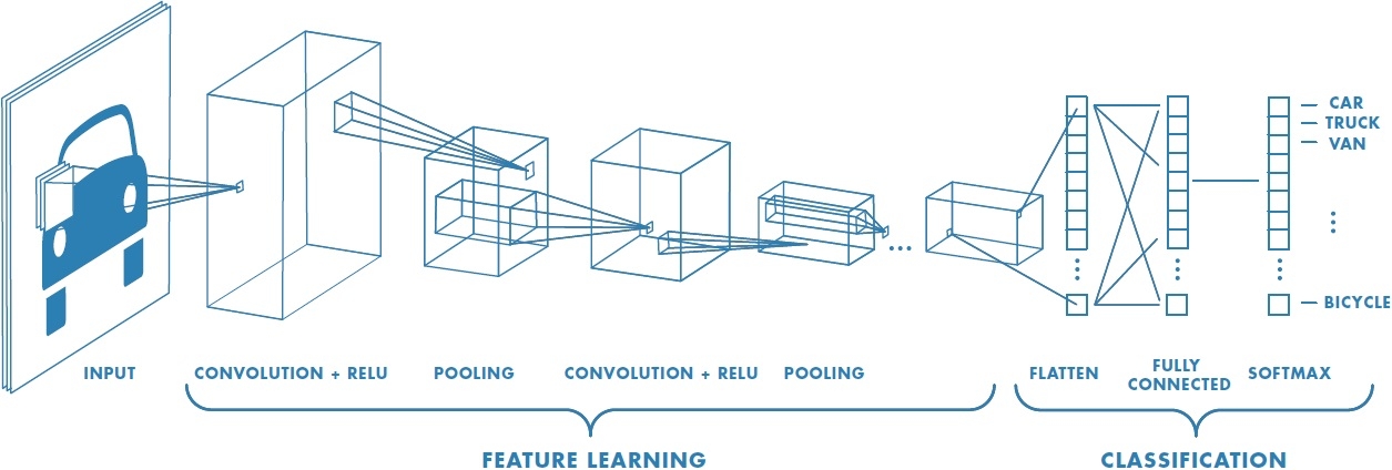
At the end of each filter layer, we typically apply a ReLU activation function. There may be multiple filter plus ReLU layers. Then we have a max pooling layer. Then we have some more filter + ReLU layers. Then we have max pooling again. Once the output is down to a relatively small size, there is typically a last fully-connected layer, leading into an activation function such as softmax that produces the final output. The exact design of these structures is an art—there is not currently any clear theoretical (or even systematic empirical) understanding of how these various design choices affect overall performance of the network.
The critical point for us is that this is all just a big neural network, which takes an input and computes an output. The mapping is a differentiable function of the weights, which means we can adjust the weights to decrease the loss by performing gradient descent, and we can compute the relevant gradients using back-propagation!
Well, technically the derivative does not exist at every point, both because of the ReLU and the max pooling operations, but we ignore that fact.
7.4 Backpropagation in a simple CNN
Let’s work through a very simple example of how back-propagation can work on a convolutional network. The architecture is shown below. Assume we have a one-dimensional single-channel image \(X\) of size \(n \times 1 \times 1\), and a single filter \(W^1\) of size \(k \times 1 \times 1\) (where we omit the filter bias) for the first convolutional operation denoted “conv” in the figure below. Then we pass the intermediate result \(Z^1\) through a ReLU layer to obtain the activation \(A^1\), and finally through a fully-connected layer with weights \(W^2\), denoted “fc” below, with no additional activation function, resulting in the output \(A^2\).
 rectangle (1,9);
\node at (.5, -2) {$X = A^0$};
\draw (0,-1) rectangle (1,0);
\draw (0,9) rectangle (1,10);
\node[anchor=center] at (0.5,-.5) {0};
\node[anchor=center] at (0.5,9.5) {0};
\node[left] at (0,-0.5) {\begin{tabular}{c}
pad with 0's \\ (to get output\\ of same shape)\end{tabular}};
\draw (3,4.5) rectangle (4,7.5);
\draw[gray] (1,9) -- (3,7.5);
\draw[gray] (1,0) -- (3,4.5);
\node at (3.5,3.5) {$W^1$};
\draw (8,0) rectangle (9,9);
\node at (8.5,-1) {$Z^1$};
\draw (12,0) rectangle (13,9);
\node at (12.5,-1) {$A^1$};
\draw (16,5.5) rectangle (17,6.5);
\node at (16.5, 4.0) {$Z^2=A^2$};
\node at (14.5,5.3) {$W^2$};
\draw[->,thick] (4.5,6) -- node[above] {conv} (7.5,6);
\draw[->,thick] (9.5,6) -- node[above] {ReLU} (11.5,6);
\draw[->,thick] (13.5,6) -- node[above] {fc} (15.5,6);
\end{tikzpicture}")
For simplicity assume \(k\) is odd, let the input image \(X = A^0\), and assume we are using squared loss. Then we can describe the forward pass as follows: \[\begin{aligned} Z_i^1 & = {W^1}^TA^0_{[i-\lfloor k/2 \rfloor : i + \lfloor k/2 \rfloor]} \\ A^1 & = ReLU(Z^1) \\ A^2 & = Z^2 = {W^2}^T A^1 \\ \mathcal{L}_{square}(A^2, y) & = (A^2-y)^2 \end{aligned}\]
Assuming a stride of \(1,\) for a filter of size \(k\), how much padding do we need to add to the top and bottom of the image? We see one zero at the top and bottom in the figure just above; what filter size is implicitly being shown in the figure? (Recall the padding is for the sake of getting an output the same size as the input.)
7.4.1 Weight update
How do we update the weights in filter \(W^1\)?
\[ \frac{\partial \text{loss}}{\partial W^1} = \frac{\partial Z^1}{\partial W^1} \frac{\partial A^1}{\partial Z^1} \frac{\partial \text{loss}}{\partial A^1} \]
\(\partial Z^1/\partial W^1\) is the \(k \times n\) matrix such that \(\partial Z_i^1/\partial W_j^1 = X_{i-\lfloor k/2 \rfloor+j-1}\). So, for example, if \(i = 10\), which corresponds to column 10 in this matrix, which illustrates the dependence of pixel 10 of the output image on the weights, and if \(k = 5\), then the elements in column 10 will be \(X_8, X_9, X_{10}, X_{11}, X_{12}\).
\(\partial A^1/\partial Z^1\) is the \(n \times n\) diagonal matrix such that
\[ \begin{aligned} \partial A_i^1/\partial Z_i^1= \begin{cases} 1 & \text{if $Z_i^1 > 0$}\\ 0 & \text{otherwise} \end{cases} \end{aligned} \]
- \(\partial \text{loss}/{\partial A^1} = (\partial \text{loss} / {\partial A^2}) (\partial A^2 / {\partial A^1}) = 2(A^2 - y)W^2\), an \(n \times 1\) vector
Multiplying these components yields the desired gradient, of shape \(k \times 1\).
7.4.2 Max pooling
One last point is how to handle back-propagation through a max-pooling operation. Let’s study this via a simple example. Imagine \[y = \max(a_1, a_2)\;\;,\] where \(a_1\) and \(a_2\) are each computed by some network. Consider doing back-propagation through the maximum. First consider the case where \(a_1 > a_2\). Then the error value at \(y\) is propagated back entirely to the network computing the value \(a_1\). The weights in the network computing \(a_1\) will ultimately be adjusted, and the network computing \(a_2\) will be untouched.
What is \(\nabla_{(x, y)} \max(x, y)\) ?