9  Transformers

Caution

We are actively overhauling the Transformers chapter from the legacy PDF notes to enhance clarity and presentation. Please feel free to raise issues or request more explanation on specific topics.

Transformers are a very recent family of architectures that were originally introduced in the field of natural language processing (NLP) in 2017, as an approach to process and understand human language. Since then, they have revolutionized not only NLP but also other domains such as image processing and multi-modal generative AI. Their scalability and parallelizability have made them the backbone of large-scale foundation models, such as GPT, BERT, and Vision Transformers (ViT), powering many state-of-the-art applications.

Human language is inherently sequential in nature (e.g., characters form words, words form sentences, and sentences form paragraphs and documents). Prior to the advent of the transformers architecture, recurrent neural networks (RNNs) briefly dominated the field for their ability to process sequential information. However, RNNs, like many other architectures, processed sequential information in an iterative/sequential fashion, whereby each item of a sequence was individually processed one after another. Transformers offer many advantages over RNNs, including their ability to process all items in a sequence in a parallel fashion (as do CNNs).

Like CNNs, transformers factorize signal processing into stages, each involving independently and identically processed chunks. Transformers have many intricate components; however, we’ll focus on their most crucial innovation: a new type of layer called the attention layer. Attention layers enable transformers to effectively mix information across chunks, allowing the entire transformer pipeline to model long-range dependencies among these chunks. To help make Transformers more digestible, in this chapter, we will first succinctly motivate and describe them in an overview Section 9.1. Then, we will dive into the details following the flow of data – first describing how to represent inputs Section 9.2, and then describe the attention mechanism Section 9.3, and finally we then assemble all these ideas together to arrive at the full transformer architecture in Section 9.5.

9.1 Transformers Overview

Transformers are powerful neural architectures designed primarily for sequential data, such as text. At their core, transformers are typically auto-regressive, meaning they generate sequences by predicting each token sequentially, conditioned on previously generated tokens. This auto-regressive property ensures that the transformer model inherently captures temporal dependencies, making them especially suited for language modeling tasks like text generation and completion.

Suppose our training data contains this sentence: “To date, the cleverest thinker was Issac.” The transformer model will learn to predict the next token in the sequence, given the previous tokens. For example, when predicting the token “cleverest,” the model will condition its prediction on the tokens “To,” “date,” and “the.” This process continues until the entire sequence is generated.

The animation above illustrates the auto-regressive nature of transformers.

Below is another example. Suppose the sentence is the 2nd law of robotics: “A robot must obey the orders given it by human beings…” The training objective of a transformer would be to make each token’s prediction, conditioning on previously generated tokens, forming a step-by-step probability distribution over the vocabulary.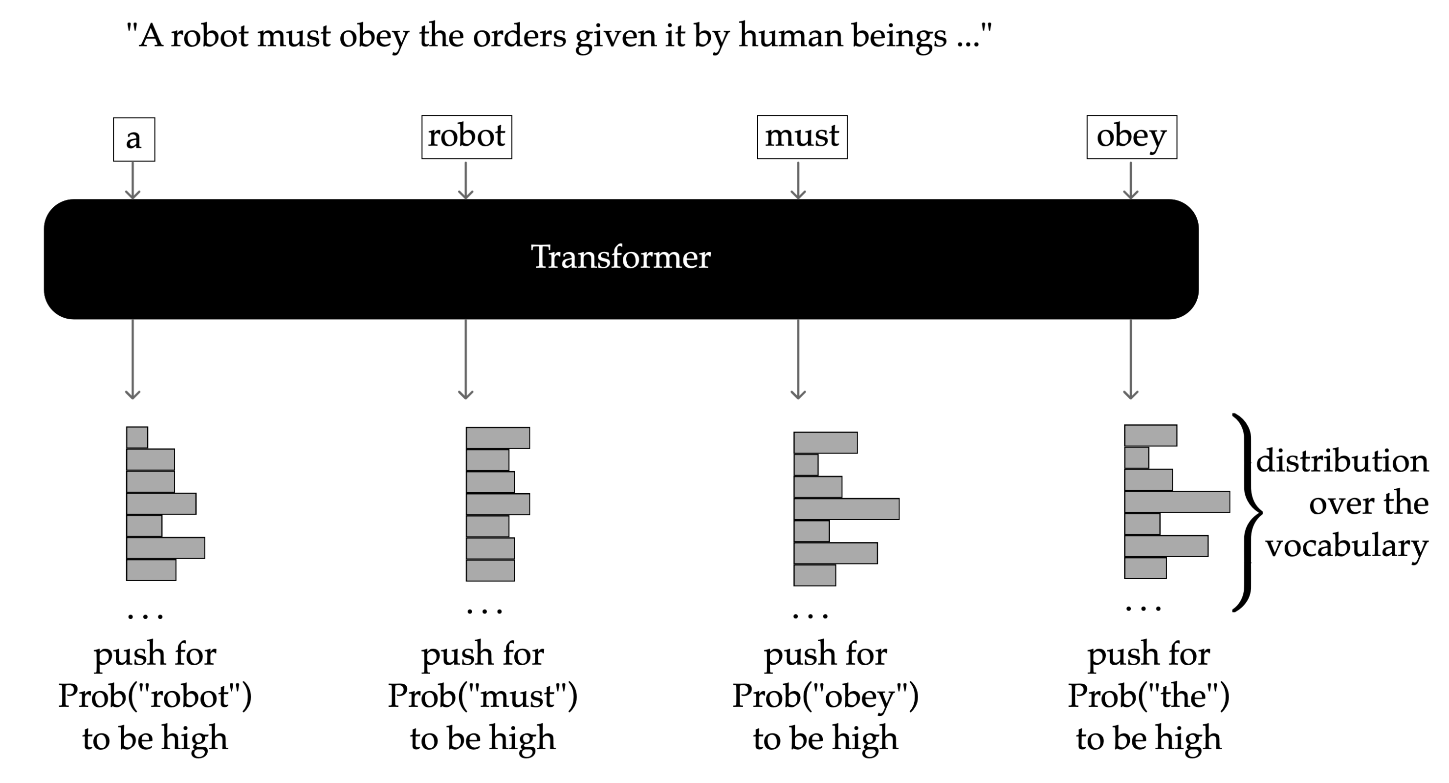

The transformer architecture processes inputs by applying multiple identical building blocks stacked in layers. Each block performs a transformation that progressively refines the internal representation of the data.

Specifically, each block consists of two primary sub-layers: an attention layer Section 9.4 and a feed-forward network (or multi-layer perceptron) Chapter 6. Attention layers mix information across different positions (or "chunks") in the sequence, allowing the model to effectively capture dependencies regardless of distance. Meanwhile, the feed-forward network significantly enhances the expressiveness of these representations by applying non-linear transformations independently to each position.

A notable strength of transformers is their capacity for parallel processing. Transformers process entire sequences simultaneously rather than sequentially token-by-token. This parallelization significantly boosts computational efficiency and makes it feasible to train larger and deeper models.

In this overview, we emphasize the auto-regressive nature of transformers, their layered approach to transforming representations, the parallel processing advantage, and the critical role of the feed-forward layers in enhancing their expressive power.

There are additional essential components and enhancements—such as causal attention mechanisms and positional encoding—that further empower transformers. We’ll explore these "bells and whistles" in greater depth in subsequent discussions.

9.2 Embedding and Representations

We start by describing how language is commonly represented, then we provide a brief explanation of why it can be useful to predict subsequent items (e.g., words/tokens) in a sequence.

As a reminder, two key components of any ML system are: (1) the representation of the data; and (2) the actual modelling to perform some desired task. Computers, by default, have no natural way of representing human language. Modern computers are based on the Von Neumann architecture and are essentially very powerful calculators, with no natural understanding of what any particular string of characters means to us humans. Considering the rich complexities of language (e.g., humor, sarcasm, social and cultural references and implications, slang, homonyms, etc), you can imagine the innate difficulties of appropriately representing languages, along with the challenges for computers to then model and “understand” language.

The field of NLP aims to represent words with vectors of floating-point numbers (aka word embeddings) such that they capture semantic meaning. More precisely, the degree to which any two words are related in the ‘real-world’ to us humans should be reflected by their corresponding vectors (in terms of their numeric values). So, words such as ‘dog’ and ‘cat’ should be represented by vectors that are more similar to one another than, say, ‘cat’ and ‘table’ are.

To measure how similar any two word embeddings are (in terms of their numeric values) it is common to use some similarity as the metric, e.g. the dot-product similarity we saw in Chapter 8.

Thus, one can imagine plotting every word embedding in \(d\)-dimensional space and observing natural clusters to form, whereby similar words (e.g., synonyms) are located near each other. The problem of determining how to parse (aka tokenize) individual words is known as tokenization. This is an entire topic of its own, so we will not dive into the full details here. However, the high-level idea of tokenization is straightforward: the individual inputs of data that are represented and processed by a model are referred to as tokens. And, instead of processing each word as a whole, words are typically split into smaller, meaningful pieces (akin to syllables). For example, the word “evaluation” may be input into a model as 3 individual tokens (eval + ua + tion). Thus, when we refer to tokens, know that we’re referring to these sub-word units. For any given application/model, all of the language data must be predefined by a finite vocabulary of valid tokens (typically on the order of 40,000 distinct tokens).

How can we define an optimal vocabulary of such tokens? How many distinct tokens should we have in our vocabulary? How should we handle digits or other punctuation? How does this work for non-English languages, in particular, script-based languages where word boundaries are less obvious (e.g., Chinese or Japanese)? All of these are open NLP research problems receiving increased attention lately.

9.3 Query, Key, Value, and Attention Output

Attention mechanisms efficiently process global information by selectively focusing on the most relevant parts of the input. Given an input sentence, each token is processed sequentially to predict subsequent tokens. As more context (previous tokens) accumulates, this context ideally becomes increasingly beneficial—provided the model can appropriately utilize it. Transformers employ a mechanism known as attention, which enables models to identify and prioritize contextually relevant tokens.

For example, consider the partial sentence: “Anqi forgot ___“. At this point, the model has processed tokens”Anqi” and “forgot,” and aims to predict the next token. Numerous valid completions exist, such as articles (“the,” “an”), prepositions (“to,” “about”), or possessive pronouns (“her,” “his,” “their”). A well-trained model should assign higher probabilities to contextually relevant tokens, such as “her,” based on the feminine-associated name “Anqi.” Attention mechanisms guide the model to selectively focus on these relevant contextual cues using query, key, and value vectors.

9.3.1 Query Vectors

Our goal is for each input token to learn how much attention it should give to every other token in the sequence. To achieve this, each token is assigned a unique query vector used to “probe” or assess other tokens—including itself—to determine relevance.

A token’s query vector \(q_i\) is computed by multiplying the input token \(x_i\) (a \(d\)-dimensional vector) by a learnable query weight matrix \(W_q\) (of dimension \(d \times d_k\), \(d_k\) is a hyperparameter typically chosen such that \(d_k < d\)):

\[ q_i = W_q^T x_i \]

Thus, for a sequence of \(n\) tokens, we generate \(n\) distinct query vectors.

9.3.2 Key Vectors

To complement query vectors, we introduce key vectors, which tokens use to “answer” queries about their relevance. Specifically, when evaluating token \(x_3\), its query vector \(q_3\) is compared to each token’s key vector \(k_j\) to determine the attention weight. Each key vector \(k_i\) is computed similarly using a learnable key weight matrix \(W_k\):

\[ k_i = W_k^T x_i \]

The attention mechanism calculates similarity using the dot product, which efficiently measures vector similarity:

\[ a_i = \text{softmax}\left(\frac{[q_i^T k_1, q_i^T k_2, \dots, q_i^T k_n]}{\sqrt{d_k}}\right)^T \in \mathbb{R}^{1\times n} \]

The vector \(a_i\) (softmax’d attention scores) quantifies how much attention token \(q_i\) should pay to each token in the sequence, normalized so that elements sum to 1. Normalizing by \(\sqrt{d_k}\) prevents large dot-product magnitudes, stabilizing training.

9.3.3 Value Vectors

To incorporate meaningful contributions from attended tokens, we use value vectors (\(v_i\)), providing distinct representations for contribution to attention outputs. Each token’s value vector is computed with another learnable matrix \(W_v\):

\[ v_i = W_v^T x_i \]

9.3.4 Attention Output

Finally, attention outputs are computed as weighted sums of value vectors, using the softmax’d attention scores:

\[ z_i = \sum_{j=1}^n a_{ij} v_j \in \mathbb{R}^{d_k} \]

This vector \(z_i\) represents token \(x_i\)’s enriched embedding, incorporating context from across the sequence, weighted by learned attention.

9.4 Self-attention Layer

Self-attention is an attention mechanism where the keys, values, and queries are all generated from the same input.

At a very high level, typical transformer with self-attention layers maps \(\mathbb{R}^{n\times d} \longrightarrow \mathbb{R}^{n\times d}\). In particular, the transformer takes in \(n\) tokens, each having feature dimension \(d,\) and through many layers of transformation (most important of which are self-attention layers); the transformer finally outputs a sequence of \(n\) tokens, each of which \(d\)-dimensional still.

With a self-attention layer, there can be multiple attention head. We start with understanding a single head.

9.4.1 A Single Self-attention Head

A single self-attention head is largely the same as our discussion in Section 9.3. The main additional info introduced in this part is a compact matrix form. The layer takes in \(n\) tokens, each having feature dimension \(d\). Thus, all tokens can be collectively written as \(X\in \mathbb{R}^{n\times d}\), where the \(i\)-th row of \(X\) stores the \(i\)-th token, denoted as \(x_i\in\mathbb{R}^{1\times d}\). For each token \(x^i\), self-attention computes (via learned projection matrices, discussed in Section 9.3), a query \(q_i \in \mathbb{R}^{d_q}\), key \(k_{i} \in \mathbb{R}^{d_k}\), and value \(v_{i} \in \mathbb{R}^{d_v}\), and overall, we will have \(n\) queries, \(n\) keys, and \(n\) values; all of these vectors live in the same dimension in practice, and we often denote all three embedding dimension via a unified \(d_k\).

The self-attention output is calculated as a weighted sum:

\[ {z}_i = \sum_{j=1}^n a_{ij} v_{j}\in\mathbb{R}^{d_k } \]where \(a_{ij}\) is the \(j\)th element in \(a_i\).

So far, we’ve discussed self-attention focusing on a single token input-output. Actually, we can calculate all outputs \(z_i\) (\(i=1,2,\ldots,n\)) at the same time using a matrix form. For clearness, we first introduce the \(Q\in\mathbb{R}^{n\times d_k}\) query matrix, \(K\in\mathbb{R}^{n\times d_k}\) key matrix, and \(V\in\mathbb{R}^{n\times d_k}\) value matrix:

\[ \begin{aligned} Q &= \begin{bmatrix} q_1^\top \\ q_2^\top \\ \vdots \\ q_n^\top \end{bmatrix} \in \mathbb{R}^{n \times d}, \quad K = \begin{bmatrix} k_1^\top \\ k_2^\top \\ \vdots \\ k_n^\top \end{bmatrix} \in \mathbb{R}^{n \times d}, \quad V = \begin{bmatrix} v_1^\top \\ v_2^\top \\ \vdots \\ v_n^\top \end{bmatrix} \in \mathbb{R}^{n \times d_v} \end{aligned} \]It should be straightforward to understand that the \(Q\), \(K\), \(V\) matrices simply stack \(q_i\), \(k_i\), and \(v_i\) in a row-wise manner, respectively. Now, the the full attention matrix \(A \in \mathbb{R}^{n \times n}\) is:

\[\begin{aligned} A = \begin{bmatrix} \text{softmax}\left( \begin{bmatrix} q_1^\top k_1 & q_1^\top k_2 & \cdots & q_1^\top k_{n} \end{bmatrix} / \sqrt{d_k} \right) \\ \text{softmax}\left( \begin{bmatrix} q_2^\top k_1 & q_2^\top k_2 & \cdots & q_2^\top k_{n} \end{bmatrix} / \sqrt{d_k} \right) \\ \vdots & \\ \text{softmax}\left( \begin{bmatrix} q_{n}^\top k_1 & q_{n}^\top k_2 & \cdots & q_{n}^\top k_{n} \end{bmatrix} / \sqrt{d_k} \right) \end{bmatrix} \end{aligned} \tag{9.1}\]

which often time is shorten as: \[\begin{aligned} A = \text{softmax}\left( \frac{1}{\sqrt{d_k}} \begin{bmatrix} q_1^\top k_1 & q_1^\top k_2 & \cdots & q_1^\top k_n \\ q_2^\top k_1 & q_2^\top k_2 & \cdots & q_2^\top k_n \\ \vdots & \vdots & \ddots & \vdots \\ q_n^\top k_1 & q_n^\top k_2 & \cdots & q_n^\top k_n \end{bmatrix} \right)\end{aligned}=\text{softmax}\left(\frac{QK^\top}{\sqrt{d_k}}\right) \]

Note that the Softmax operation is applied in a row-wise manner. The \(i\)th row \(A\) of this matrix corresponds to the softmax’d attention scores computed for query \(q_i\) over all keys (i.e., \(\alpha_i\)). The full output of the self-attention layer can then be written compactly as:

\[ Z = \begin{bmatrix} z_1^\top \\ z_2^\top \\ \vdots \\ z_n^\top \end{bmatrix} = AV \in \mathbb{R}^{n \times d_k} \]

where \(V\in \mathbb{R}^{n \times d_k}\) is the matrix of value vectors stacked row-wise, and \(Z \in \mathbb{R}^{n \times d_k}\) is the output, whose \(i\)th row corresponds to the attention output for the \(i\)th query (i.e., \(z_i\)).

You will also see this compact notation Attention in the literature, which is an operation of three arguments \(Q\), \(K\), and \(V\) (and we add an emphasis that the softmax is performed on each row):

\[ \text{Attention}(Q, K, V) = \text{softmax}_{row}\left(\frac{Q K^\top}{\sqrt{d_k}}\right)V \]

9.4.2 Multi-head Self-attention

Human language can be very nuanced. There are many properties of language that collectively contribute to a human’s understanding of any given sentence. For example, words have different tenses (past, present, future, etc), genders, abbreviations, slang references, implied words or meanings, cultural references, situational relevance, etc. While the attention mechanism allows us to appropriately focus on tokens in the input sentence, it’s unreasonable to expect a single set of \(\{Q,K,V\}\) matrices to fully represent – and for a model to capture – the meaning of a sentence with all of its complexities.

To address this limitation, the idea of multi-head attention is introduced. Instead of relying on just one attention head (i.e., a single set of \(\{Q, K, V\}\) matrices), the model uses multiple attention heads, each with its own independently learned set of \(\{Q, K, V\}\) matrices. This allows each head to attend to different parts of the input tokens and to model different types of semantic relationships. For instance, one head might focus on syntactic structure and another on verb tense or sentiment. These different “perspectives” are then concatenated and projected to produce a richer, more expressive representation of the input.

Now, we introduce the formal math notations. Let us denote the number of head as \(H\). For the \(h\)th head, the input \(X \in \mathbb{R}^{n \times d}\) is linearly projected into query, key, and value matrices using the projection matrices \(W_q^{h}\in\mathbb{R}^{d\times d_q}\), \(W_k^{h}\in\mathbb{R}^{d\times d_k}\), and \(W_v^{h}\in\mathbb{R}^{d\times d_v}\) (recall that usually \(d_q=d_k=d_v\)):

\[ \begin{aligned} Q^{h} &= X W_q^{h} \\ K^{h} &= X W_k^{h} \\ V^{h} &= X W_v^{h} \end{aligned} \]

The output of the \(i\)-th head is \(Z^{h}\): \({Z}^h = \text{Attention}(Q^{h}, K^{h}, V^{h})\in\mathbb{R}^{n\times d_k}\). After computing all \(h\) heads, we concatenate their outputs and apply a final linear projection: \[ \text{MultiHead}(X) = \text{Concat}(Z^1, \dots, Z^H) W^O \] where the concatenation operation concatenates \(Z^h\) horizontally, yielding a matrix of size \(n\times Hd_k\), and \(W^O \in \mathbb{R}^{d\times Hd_k}\) is a final linear projection matrix.

9.5 Transformers Architecture Details

9.5.1 Positional Embeddings

An extremely observant reader might have been suspicious of a small but very important detail that we have not yet discussed: the attention mechanism, as introduced so far, does not encode the order of the input tokens. For instance, when computing softmax’d attention scores and building token representations, the model is fundamentally permutation-equivariant — the same set of tokens, even if scrambled into a different order, would result in identical outputs permuted in the same order — Formally, when we fix \(\{W_q,W_k,W_v\}\) and switch the input \(x_i\) with \(x_j\), then the output \(z_i\) and \(z_j\) will be switched. However, natural language is not a bag of words: meaning is tied closely to word order.

To address this, transformers incorporate positional embeddings — additional information that encodes the position of each token in the sequence. These embeddings are added to the input token embeddings before any attention layers are applied, effectively injecting ordering information into the model.

There are two main strategies for positional embeddings: (i) learned positional embeddings, where a trainable vector \(p_i\in\mathbb{R}^d\) is assigned to each position (i.e., token index) \(i=0, 1, 2, ..., n\). These vectors are learned alongside all other model parameters and allow the model to discover how best to encode position for a given task, (ii) fixed positional embeddings, such as sinusoidal positional embedding proposed in the original Transformer paper:

\[ \begin{aligned} p_{(i, 2k)} = \sin\left( \frac{i}{10000^{2k/d}} \right) \\ p_{(i, 2k+1)} = \cos\left( \frac{i}{10000^{2k/d}} \right) \end{aligned} \]

where \(i=1,2,..,n\) is the token index, while \(k=1,2,...,d\) is the dimension index. Namely, this sinusoidal positional embedding uses sine for the even dimension and cosine for the odd dimension. Regardless of learnable or fixed positional embedding, it will enter the computation of attention at the input place: \(x_i^*=x_i+p_i~,\)​ where \(x_i\) is the \(i\)th original input token, and \(p_i\) is its positional embedding. The \(x_i^*\) will now be what we really feed into the attention layer, so that the input to the attention mechanism now carries information about both what the token is and where it appears in the sequence.

This simple additive design enables attention layers to leverage both semantic content and ordering structure when deciding where to focus. In practice, this addition occurs at the very first layer of the transformer stack, and all subsequent layers operate on position-aware representations. This is a key design choice that allows transformers to work effectively with sequences of text, audio, or even image patches (as in Vision Transformers).

9.5.2 Causal Self-attention

More generally, a mask may be applied to limit which tokens are used in the attention computation. For example, one common mask limits the attention computation to tokens that occur previously in time to the one being used for the query. This prevents the attention mechanism from “looking ahead” in scenarios where the transformer is being used to generate one token at a time. This causal masking is done by introducing a mask matrix \(M \in \mathbb{R}^{n \times n}\) that restricts attention to only current and previous positions. A typical causal mask is a lower-triangular matrix:

\[ M = \begin{bmatrix} 0 & -\infty & -\infty & \cdots & -\infty \\ 0 & 0 & -\infty & \cdots & -\infty \\ 0 & 0 & 0 & \cdots & -\infty \\ \vdots & \vdots & \vdots & \ddots & \vdots \\ 0 & 0 & 0 & \cdots & 0 \end{bmatrix} \]

and we now have the masked attention matrix:

\[\begin{aligned} A = \text{softmax}\left( \frac{1}{\sqrt{d_k}} \begin{bmatrix} q_1^\top k_1 & q_1^\top k_2 & \cdots & q_1^\top k_n \\ q_2^\top k_1 & q_2^\top k_2 & \cdots & q_2^\top k_n \\ \vdots & \vdots & \ddots & \vdots \\ q_n^\top k_1 & q_n^\top k_2 & \cdots & q_n^\top k_n \end{bmatrix} + M \right)\end{aligned} \] The softmax is performed to each row independently. The attention output is still \(Y= A V\). Essentially, the lower-triangular property of \(M\) ensures that the self-attention operation for the \(j\)-th query only considers tokens \(0,1,...,j\). Note that we should apply the masking before performing softmax, so that the attention matrix can be properly normalized (i.e., each row sum to 1).

Each self-attention stage is trained to have key, value, and query embeddings that lead it to pay specific attention to some particular feature of the input. We generally want to pay attention to many different kinds of features in the input; for example, in translation one feature might be be the verbs, and another might be objects or subjects. A transformer utilizes multiple instances of self-attention, each known as an “attention head,” to allow combinations of attention paid to many different features.