Introduction to Machine Learning

Due: Monday, February 13, 2023 at 11:00 PM

Lab attendance check

Type in your section passcode to get attendance credit
(normally within the first 15 minutes of your scheduled section; but today only, passcode is accepted anytime in-session.)
Passcode:  Enter

Ask for Help Loading...

Instructions

In 6.390 a large part of the learning happens by discussing lab questions with partners. Please complete this group self-partnering question then begin the lab.

Create/join a group

1. One person (and only one) should create a group.

   New group name: Submit

2. Everyone else should enter the group name below (in the form groupname_0000).

   Join group: Submit

To join another group or leave your current group, reload the page.

You are not in a group.

Ask for Help Loading...

Lab: Random Hypotheses

In this lab we will experiment with a simple algorithm for trying to find a line that fits well a set of data \mathcal{D}_n=\left\{\left(x^{(1)}, y^{(1)}\right), \ldots,\left(x^{(n)}, y^{(n)}\right)\right\} where x^{(i)}\in \mathbb{R}. We will generate a lot of random hypotheses within linear hypothesis class-- i.e., a lot of models with the same linear parametrization but each with randomly generated parameters; or more specifically in this case, a lot of lines, each with randomly generated slope and intercept.

We will then see which one has the smallest error on this data, and return that one as our answer. We don't recommend this method in actual practice, but it gets us started and makes some useful points.

Note that this lab builds on the lecture notes Chapter 1 - Intro to ML and Chapter 2 - Regression for background and terminology, and the algorithm itself is a version of the random-regression algorithm from the notes Section 2.4. The second part of Homework 1 asks you about the implementation of a similar version, so this lab will also help get you ready for the homework!

It is good practice for you and your team to write down short answers to the lab questions as you work through them so that you are prepared for a check-off conversation at the end.

Here is the top-level code for the algorithm (random_regress(X, Y, k)) presented below:

• X is a d \times n matrix with n training input points in a d-dimensional space.
• Y is a 1 \times n vector with n training output values.
• k is the number of random hypotheses to try.

All of this is normal Python and numpy, except the procedure lin_reg_err, which you will implement in Homework 1 (where you will also learn numpy!). It takes in the training data, and k hypotheses (in the ths and th0ss arrays) and returns a vector of k values of the mean squared error (MSE) of each of the hypotheses on the data.

In particular, consider one hypothesis (out of the k possible hypotheses). Suppose this hypothesis' parameters are \theta and \theta_0, then its MSE is defined as

where g^{(i)}=\theta^T x^{(i)} + \theta_0 is the prediction or guess by the hypothesis for sample i, and y^{(i)} is the actual label for sample i.

def random_regress(X, Y, k):
    d, n = X.shape

    # generate k random hypotheses
    ths = np.random.randn(d, k)
    th0s = np.random.randn(1, k)

    # compute the mean squared error of each hypothesis on the data set
    errors = lin_reg_err(X, Y, ths, th0s.T)

    # Find the index of the hypotheses with the lowest error
    i = np.argmin(errors)

    # return the theta and theta0 parameters that define that hypothesis
    theta, theta0 = ths[:,i:i+1], th0s[:,i:i+1]
    return (theta, theta0), errors[i]

You'll get more practice with numpy in the homework, but in the meantime you might find the numpy reference for np.random.randn helpful.

Talk through this code with your group, and try to get a basic understanding of what is going on. Put yourself in the help queue to ask if you have any questions!

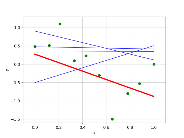
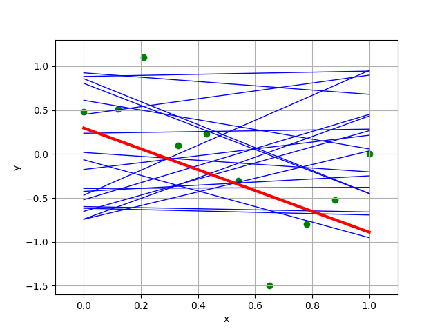
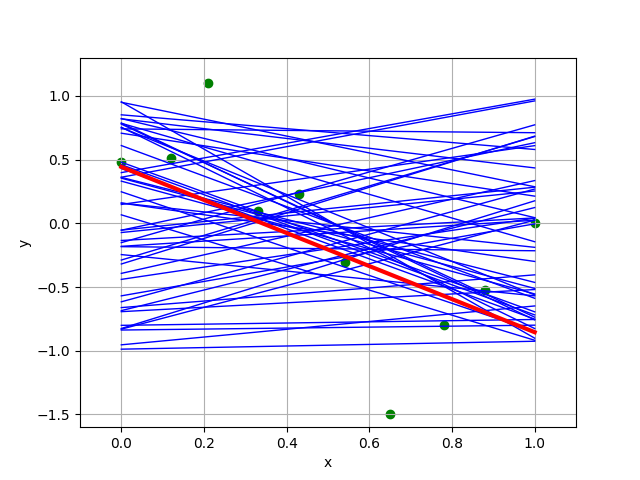
We'll start by studying example executions of this algorithm with a data set where d = 1, n = 10 for different values of k (so the horizontal axis is the single dimension of x and the vertical axis is the output y). The hypothesis with minimal mean squared error (MSE), of the k that were tested, is shown in red.

Here is the data set and one random hypothesis.

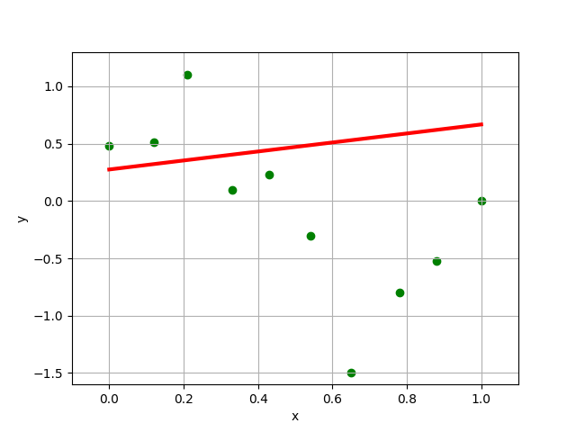
• Is this a good hypothesis?
• For all hypotheses within the linear hypothesis class (all including those we didn't get to test), which one would achieve the minimal MSE, roughly?

Now, here are some executions for different values of k (shown in red is the hypothesis with the lowest MSE, among the k tested).

• What happens as we increase k? Compare the four “best” linear regressors found by the random regression algorithm with different values of k chosen, which one does your group think is "best of the best"?
• How does it match your initial guess about the best hypothesis?
• Will this method eventually get arbitrarily close to the best solution? What do you think about the efficiency of this method?

Evaluation

Now, we'll study how different settings of this algorithm (choice of the value of k and the amount of training data n) affect its performance.

We have an experimental procedure(n, m, d, k) that works as follows:

• Generate a random regression problem with d input dimensions, which we'll use as a test for the algorithm. We do this by randomly drawing some hidden parameters \theta and \theta_0 which the learning algorithm will not get to observe.

• Generate a data set (X, Y) with (n+m) data points. The X values are drawn uniformly from range [0, 1]. The output vector Y contains \theta^T x^{(i)} + \theta_0 + \epsilon^{(i)} for each column vector x^{(i)} in X, where \epsilon^{(i)} is some small random noise.

• Randomly split the data set into two parts, the training set containing n data points, and the validation set containing m data points.

• Run the random_regress(X, Y, k) algorithm on the training set to get estimated \theta and \theta_0.

• Compute the MSE of \theta, \theta_0 on the validation set (which the learning algorithm didn't get to see).

Talk through this algorithm with your partner to be sure it makes sense. For instance, what should be the dimensions of \theta and \theta_0?

We will study some plots that show the performance of this algorithm and try to explain some observations we make of them.

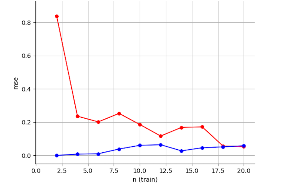
First, we'll fix m=20, d = 10, and k = 10000, and we'll run our procedure for different values of training set size n, with n ranging from 2 to 20.

The blue curve reports the mean squared error on the training set and the red curve reports it on the validation set.

For each of the following observations, come up with an explanation; you may use the Potential Explanations (below) as a set of possible ideas for answers.

• 1. With small n relative to d, and large k, the training and validation errors are substantially different, with validation error much higher. Why?
• 2. As the amount of training data increases, the training error increases slightly. Why?
• 3. As the amount of training data increases, the validation error goes down a lot. Why?

Potential Explanations

• A. With increasing training data, the learned hypothesis is more likely to be close to the true underlying hypothesis.

• B. The variation of the errors (with respect to varying k) has to do with the random sampling of hypotheses -- sometimes when we run the learning algorithm (we run it independently once per experiment) it happens to get a good hypothesis, and sometimes it doesn't.

• C. Because a small value of k is not guaranteed to generate a good hypothesis.

• D. Because the error of a hypothesis on two different, but large, data sets from the same source is likely to be very similar, independent of whether it's a good or bad hypothesis.

• E. Because with just a few points in a high-dimensional space, there are lots of different hypotheses that will have low error on the training set. This means we can generally find a hypothesis that goes near them. But when we draw a new set of points, they might be very far away from our hypothesis.

• F. Because it is easier to get a small training error when you have a lot of parameters relative to the amount of training data.

Now, we'll fix m=500, n = 500 and d = 3, and we'll run our procedure for different values of k, with k ranging from 1 to 20.

The blue curve reports the mean squared error on the training set and the red curve reports it on the validation set.

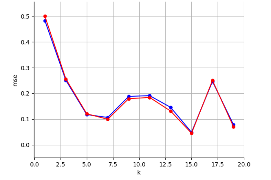
For each of the following observations, come up with an explanation; you may use the Potential Explanations (below) as a set of possible ideas for answers.

• 1. With large n relative to d, the training and validation errors are very similar. Why?
• 2. Note how much smaller our k’s are in this plot compared to part 2.2 where k = 10000. With smaller k, why do the curves go up and down so much?

Potential Explanations

• A. With increasing training data, the learned hypothesis is more likely to be close to the true underlying hypothesis.

• B. The variation of the errors (with respect to varying k) has to do with the random sampling of hypotheses -- sometimes when we run the learning algorithm (we run it independently once per experiment) it happens to get a good hypothesis, and sometimes it doesn't.

• C. Because a small value of k is not guaranteed to generate a good hypothesis.

• D. Because the error of a hypothesis on two different, but large, data sets from the same source is likely to be very similar, independent of whether it's a good or bad hypothesis.

• E. Because with just a few points in a high-dimensional space, there are lots of different hypotheses that will have low error on the training set. This means we can generally find a hypothesis that goes near them. But when we draw a new set of points, they might be very far away from our hypothesis.

• F. Because it is easier to get a small training error when you have a lot of parameters relative to the amount of training data.

<section*>Checkoff</section*> Note that only one person per team needs to get into the queue for the checkoff, if you are doing the checkoff during lab time. You do not have to finish the checkoff during lab -- lab checkoffs are typically due the following Monday at 11pm.

Checkoff:
Have a check-off conversation with a staff member; mainly for us to get some facetime with each other 😉. We would also love to chat a bit about the lab and all the questions above.

Ask for Help Ask for Checkoff Loading...

Survey

(The form below is to help us improve/calibrate for future assignments; submission is encouraged but not required. Thanks!)