13 Clustering
This page contains all content from the legacy PDF notes; clustering chapter.
As we phase out the PDF, this page may receive updates not reflected in the static PDF.
Oftentimes a dataset can be partitioned into different categories. A doctor may notice that their patients come in cohorts and different cohorts respond to different treatments. A biologist may gain insight by identifying that bats and whales, despite outward appearances, have some underlying similarity, and both should be considered members of the same category, i.e., “mammal”. The problem of automatically identifying meaningful groupings in datasets is called clustering. Once these groupings are found, they can be leveraged toward interpreting the data and making optimal decisions for each group.
13.1 Clustering formalisms
Mathematically, clustering looks a bit like classification: we wish to find a mapping from datapoints, \(x\), to categories, \(y\). However, rather than the categories being predefined labels, the categories in clustering are automatically discovered partitions of an unlabeled dataset.
Because clustering does not learn from labeled examples, it is an example of an unsupervised learning algorithm. Instead of mimicking the mapping implicit in supervised training pairs \(\{x^{(i)},y^{(i)}\}_{i=1}^n\), clustering assigns datapoints to categories based on how the unlabeled data \(\{x^{(i)}\}_{i=1}^n\) is distributed in data space.
Intuitively, a “cluster” is a group of datapoints that are all nearby to each other and far away from other clusters. Let’s consider the following scatter plot. How many clusters do you think there are?
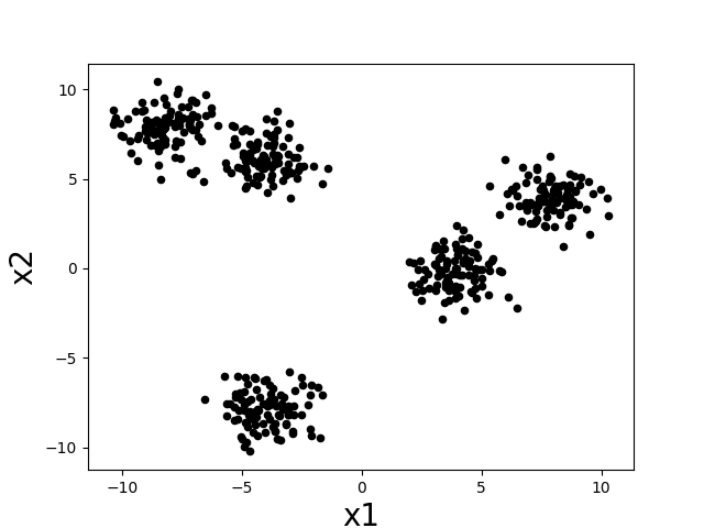
There seem to be about five clumps of datapoints and those clumps are what we would like to call clusters. If we assign all datapoints in each clump to a cluster corresponding to that clump, then we might desire that nearby datapoints are assigned to the same cluster, while far apart datapoints are assigned to different clusters.
In designing clustering algorithms, three critical things we need to decide are:
How do we measure distance between datapoints? What counts as “nearby” and “far apart”?
How many clusters should we look for?
How do we evaluate how good a clustering is?
We will see how to begin making these decisions as we work through a concrete clustering algorithm in the next section.
13.2 The k-means formulation
One of the simplest and most commonly used clustering algorithms is called k-means. The goal of the k-means algorithm is to assign datapoints to \(k\) clusters in such a way that the variance within clusters is as small as possible. Notice that this matches our intuitive idea that a cluster should be a tightly packed set of datapoints.
Similar to the way we showed that supervised learning could be formalized mathematically as the minimization of an objective function (loss function + regularization), we will show how unsupervised learning can also be formalized as minimizing an objective function. Let us denote the cluster assignment for a datapoint \(x^{(i)}\) as \(y^{(i)} \in \{1,2,\ldots,k\}\), i.e., \(y^{(i)} = 1\) means we are assigning datapoint \(x^{(i)}\) to cluster number 1. Then the k-means objective can be quantified with the following objective function (which we also call the “k-means loss”):
\[\sum_{j=1}^k \sum_{i=1}^n \mathbb{1}(y^{(i)} = j) \left\Vert x^{(i)} - \mu^{(j)} \right\Vert^2 \;, \tag{13.1}\]
where \(\mu^{(j)} = \frac{1}{N_j} \sum_{i=1}^n \mathbb{1}(y^{(i)} = j) x^{(i)}\) and \(N_j = \sum_{i=1}^n \mathbb{1}(y^{(i)} = j)\), so that \(\mu^{(j)}\) is the mean of all datapoints in cluster \(j\), and using \(\mathbb{1}(\cdot)\) to denote the indicator function (which takes on value of 1 if its argument is true and 0 otherwise). The inner sum (over data points) of the loss is the variance of datapoints within cluster \(j\). We sum up the variance of all \(k\) clusters to get our overall loss.
13.2.1 K-means algorithm
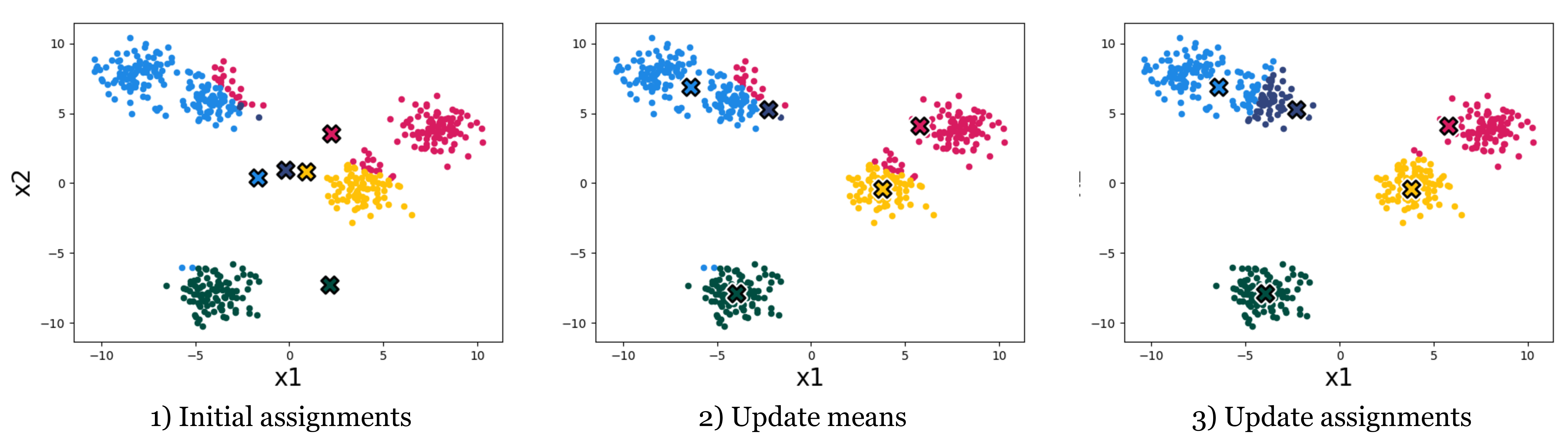
The k-means algorithm minimizes this loss by alternating between two steps: given some initial cluster assignments: 1) compute the mean of all data in each cluster and assign this as the “cluster mean”, and 2) reassign each datapoint to the cluster with nearest cluster mean. Fig. 1.2 shows what happens when we repeat these steps on the dataset from above.
Each time we reassign the data to the nearest cluster mean, the k-means loss decreases (the datapoints end up closer to their assigned cluster mean), or stays the same. And each time we recompute the cluster means the loss also decreases (the means end up closer to their assigned datapoints) or stays the same. Overall then, the clustering gets better and better, according to our objective – until it stops improving.
After four iterations of cluster assignment + update means in our example, the k-means algorithm stops improving. We say it has converged, and its final solution is shown in Fig. 1.3.
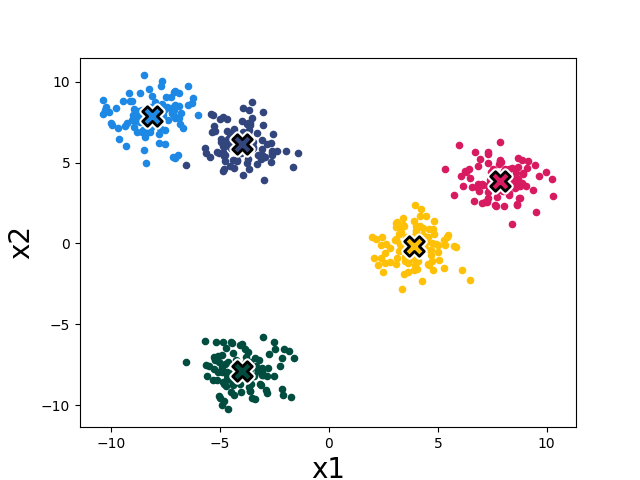
It seems to converge to something reasonable! Now let’s write out the algorithm in complete detail:
The for-loop over the \(n\) datapoints assigns each datapoint to the nearest cluster center. The for-loop over the k clusters updates the cluster center to be the mean of all datapoints currently assigned to that cluster. As suggested above, it can be shown that this algorithm reduces the loss in Equation 13.1 on each iteration, until it converges to a local minimum of the loss.
It’s like classification except it picked what the classes are rather than being given examples of what the classes are.
13.2.2 Using gradient descent to minimize k-means objective
We can also use gradient descent to optimize the k-means objective. To show how to apply gradient descent, we first rewrite the objective as a differentiable function only of \(\mu\): \[L(\mu) = \sum_{i=1}^n \min_j \left\Vert x^{(i)} - \mu^{(j)} \right\Vert^2 \;\;.\] \(L(\mu)\) is the value of the k-means loss given that we pick the optimal assignments of the datapoints to cluster means (that’s what the \(\min_j\) does). Now we can use the gradient \(\frac{\partial L(\mu)}{\partial \mu}\) to find the values for \(\mu\) that achieve minimum loss when cluster assignments are optimal. Finally, we read off the optimal cluster assignments, given the optimized \(\mu\), just by assigning datapoints to their nearest cluster mean: \[y^{(i)} = \arg\min_j \left\Vert x^{(i)} - \mu^{(j)} \right\Vert^2 \;\;.\] This procedure yields a local minimum of Equation 13.1, as does the standard k-means algorithm we presented (though they might arrive at different solutions). It might not be the global optimum since the objective is not convex (due to \(\min_j\), as the minimum of multiple convex functions is not necessarily convex).
13.2.3 Importance of initialization
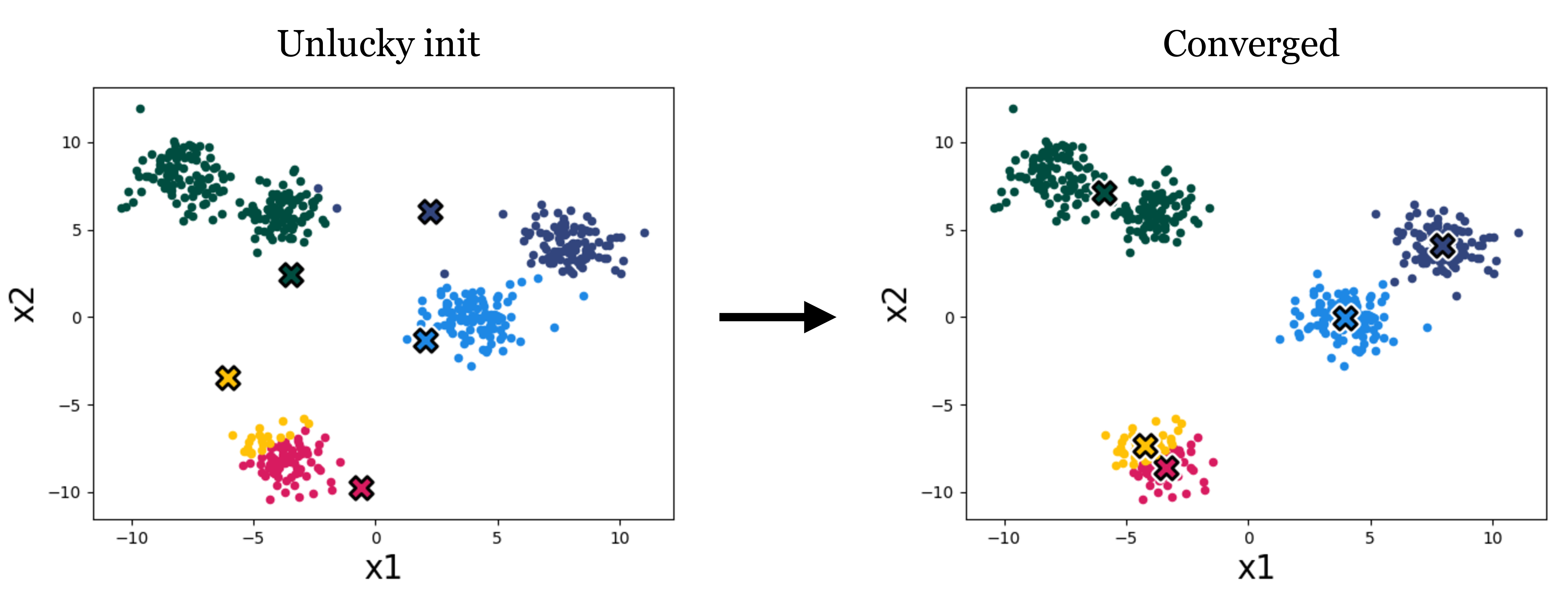
The standard k-means algorithm, as well as the variant that uses gradient descent, both are only guaranteed to converge to a local minimum, not necessarily the global minimum of the loss. Thus the answer we get out depends on how we initialize the cluster means. Figure 1.4 is an example of a different initialization on our toy data, which results in a worse converged clustering:
A variety of methods have been developed to pick good initializations (see, for example, the k-means++ algorithm). One simple option is to run the standard k-means algorithm multiple times, with different random initial conditions, and then pick from these the clustering that achieves the lowest k-means loss.
13.2.4 Importance of k
A very important parameter in cluster algorithms is the number of clusters we are looking for. Some advanced algorithms can automatically infer a suitable number of clusters, but most of the time, like with k-means, we will have to pick \(k\) – it’s a hyperparameter of the algorithm.
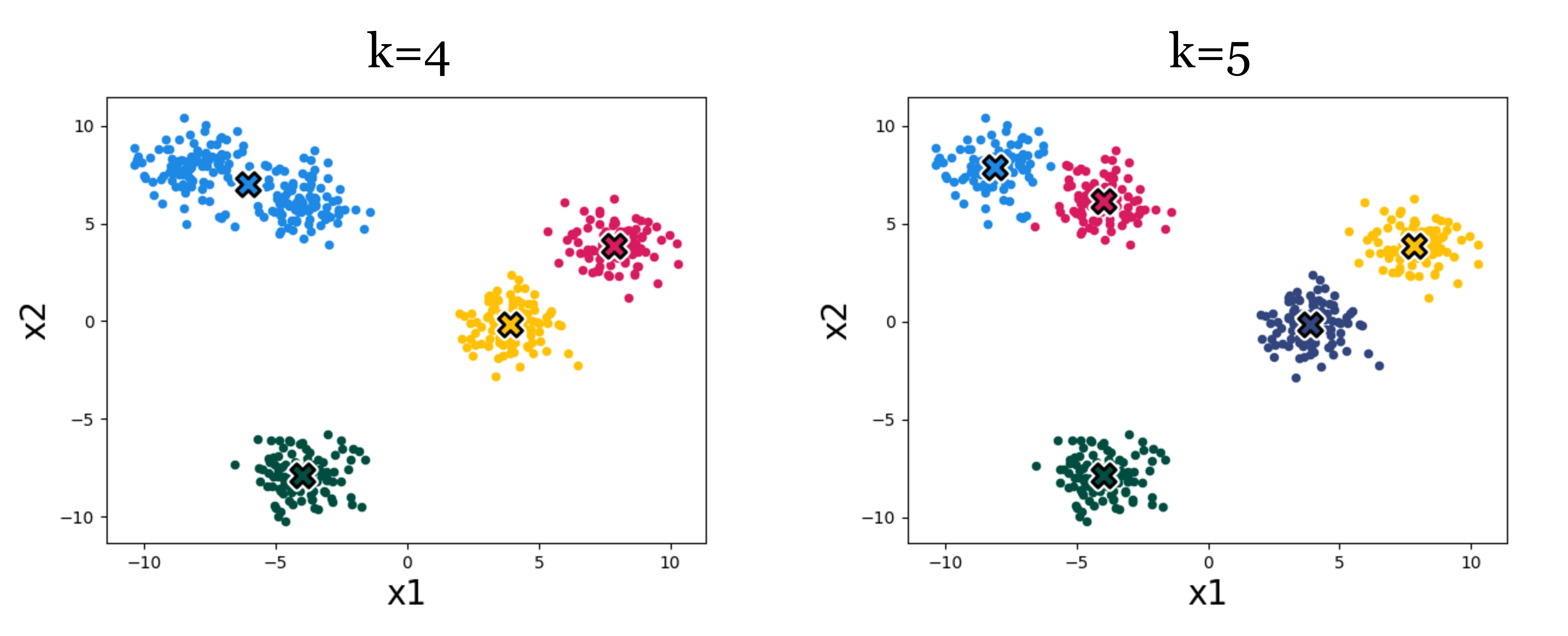
Figure 1.5 shows an example of the effect. Which result looks more correct? It can be hard to say! Using higher k we get more clusters, and with more clusters we can achieve lower within-cluster variance – the k-means objective will never increase, and will typically strictly decrease as we increase k. Eventually, we can increase k to equal the total number of datapoints, so that each datapoint is assigned to its own cluster. Then the k-means objective is zero, but the clustering reveals nothing. Clearly, then, we cannot use the k-means objective itself to choose the best value for k. In Section 1.3, we will discuss some ways of evaluating the success of clustering beyond its ability to minimize the k-means objective, and it’s with these sorts of methods that we might decide on a proper value of k.
Alternatively, you may be wondering: why bother picking a single k? Wouldn’t it be nice to reveal a hierarchy of clusterings of our data, showing both coarse and fine groupings? Indeed hierarchical clustering is another important class of clustering algorithms, beyond k-means. These methods can be useful for discovering tree-like structure in data, and they work a bit like this: initially a coarse split/clustering of the data is applied at the root of the tree, and then as we descend the tree we split and cluster the data in ever more fine-grained ways. A prototypical example of hierarchical clustering is to discover a taxonomy of life, where creatures may be grouped at multiple granularities, from species to families to kingdoms. You may find a suite of clustering algorithms in SKLEARN’s cluster module.
13.2.5 k-means in feature space
Clustering algorithms group data based on a notion of similarity, and thus we need to define a distance metric between datapoints. This notion will also be useful in other machine learning approaches, such as nearest-neighbor methods that we see in Chapter 12. In k-means and other methods, our choice of distance metric can have a big impact on the results we will find.
Our k-means algorithm uses the Euclidean distance, i.e., \(\left\Vert x^{(i)} - \mu^{(j)} \right\Vert\), with a loss function that is the square of this distance. We can modify k-means to use different distance metrics, but a more common trick is to stick with Euclidean distance but measured in a feature space. Just like we did for regression and classification problems, we can define a feature map from the data to a nicer feature representation, \(\phi(x)\), and then apply k-means to cluster the data in the feature space.
As a simple example, suppose we have two-dimensional data that is very stretched out in the first dimension and has less dynamic range in the second dimension. Then we may want to scale the dimensions so that each has similar dynamic range, prior to clustering. We could use standardization, like we did in Chapter 5.
If we want to cluster more complex data, like images, music, chemical compounds, etc., then we will usually need more sophisticated feature representations. One common practice these days is to use feature representations learned with a neural network. For example, we can use an autoencoder to compress images into feature vectors, then cluster those feature vectors.
13.3 How to evaluate clustering algorithms
One of the hardest aspects of clustering is knowing how to evaluate it. This is actually a big issue for all unsupervised learning methods, since we are just looking for patterns in the data, rather than explicitly trying to predict target values (which was the case with supervised learning).
Remember, evaluation metrics are not the same as loss functions, so we can’t just measure success by looking at the k-means loss. In prediction problems, it is critical that the evaluation is on a held-out test set, while the loss is computed over training data. If we evaluate on training data we cannot detect overfitting. Something similar is going on with the example in Section 1.2.4, where setting k to be too large can precisely “fit” the data (minimize the loss), but yields no general insight.
One way to evaluate our clusters is to look at the consistency with which they are found when we run on different subsamples of our training data, or with different hyperparameters of our clustering algorithm (e.g., initializations). For example, if running on several bootstrapped samples (random subsets of our data) results in very different clusters, it should call into question the validity of any of the individual results.
If we have some notion of what ground truth clusters should be, e.g., a few data points that we know should be in the same cluster, then we can measure whether or not our discovered clusters group these examples correctly.
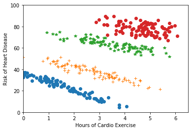
Clustering is often used for visualization and interpretability, to make it easier for humans to understand the data. Here, human judgment may guide the choice of clustering algorithm. More quantitatively, discovered clusters may be used as input to downstream tasks. For example, as we saw in the lab, we may fit a different regression function on the data within each cluster. Figure 1.6 gives an example where this might be useful. In cases like this, the success of a clustering algorithm can be indirectly measured based on the success of the downstream application (e.g., does it make the downstream predictions more accurate).